In [16]:
import folium
borders = (([-17.091, -7.443] , [122.963, 139.055]),
           ([-14.505, -10.005], [127.385, 134.693]),
           ([-13.757, -10.757], [129.557, 132.529]))
coordinates = []
for n, (lats, lons) in enumerate(borders):
    x, y =[lons[0], lons[0], lons[1],lons[1]], [lats[0], lats[1], lats[1], lats[0]]
    l = list(zip(x,y))
    l.append(l[0])
    coordinates.append(l)
geoJsonData = {
    "features": [
        {
            "geometry": {
                "coordinates": coordinates[0]
                ,
                "type": "LineString"
            },
            "properties": {
                "stroke": "#fc1717",
                "stroke-opacity": 1,
                "stroke-width": 2
            },
            "type": "Feature"
        },
        {
            "geometry": {
                "coordinates": coordinates[1]
                ,
                "type": "LineString"
            },
            "properties": {
                "stroke": "#1f1a95",
                "stroke-opacity": 1,
                "stroke-width": 2
            },
            "type": "Feature"
        },
         {
            "geometry": {
                "coordinates": coordinates[2]
                ,
                "type": "LineString"
            },
            "properties": {
                "stroke": "orange",
                "stroke-opacity": 1,
                "stroke-width": 2
            },
            "type": "Feature"
        }

    ],
    "type": "FeatureCollection"
}
todo = ('Climate Change due to Mountain Formation (COSMO CLM (50km)',
        'Coastal Convection in the Tropics: CV based Pattern Recog.',
        'SMCM: Proto-Type for Coastal Couds',
        'UM: Implement sea-breeze trigger',
        'Sub-km simulation of Island Storms',
        'Data Analysis Software Develpment')
locations=(
    (52.457739, 13.310591, 'FU Berlin', folium.Icon(color='green', prefix='fa', icon='fa-university')),
    (-37.909199, 147.131103, 'Monash Uni',  folium.Icon(color='blue',  prefix='fa', icon='fa-university')),
    (48.464822, -123.314190, 'Uni of Victoria',  folium.Icon(color='orange', prefix='fas', icon='fa-handshake')),
    (50.727208, -3.474619, 'UK Met Office',  folium.Icon(color='black', prefix='fas', icon='fa-handshake')),
    (-37.797191, 142.965023, 'Uni of Melbourne', folium.Icon(color='brown', prefix='fa', icon='fa-university')),
    (53.588599, 9.829234, 'Eu XFEL', folium.Icon(color='brown', prefix='fa', icon='database')))
m = folium.Map(location=(0,0), zoom_start=2.4)
for nn, loc in enumerate(locations):
    folium.Marker(loc[0:2], popup=todo[nn], tooltip=None, icon=loc[-1]).add_to(m)


#folium.GeoJson(geoJsonData,
#    style_function=lambda x: {
#        'color' : x['properties']['stroke'],
#        'weight' : x['properties']['stroke-width'],
#        'opacity': 0.6,
#        }).add_to(m)
display(m)
#folium.Icon?
- 10/2004 - 12/2011 : Meteorology (FU Berlin)
- 02/2012 - 03/2013 : Research Associate (FUB / DFG RiftLink)
- 05/2013 - 11/2016 : PhD (Monash Uni)
- 02/2017 - 01/2018 : Post-Doc (Monash Uni)
- 02/2018 - 12/2018 : Post-Doc (Uni Melbourne)
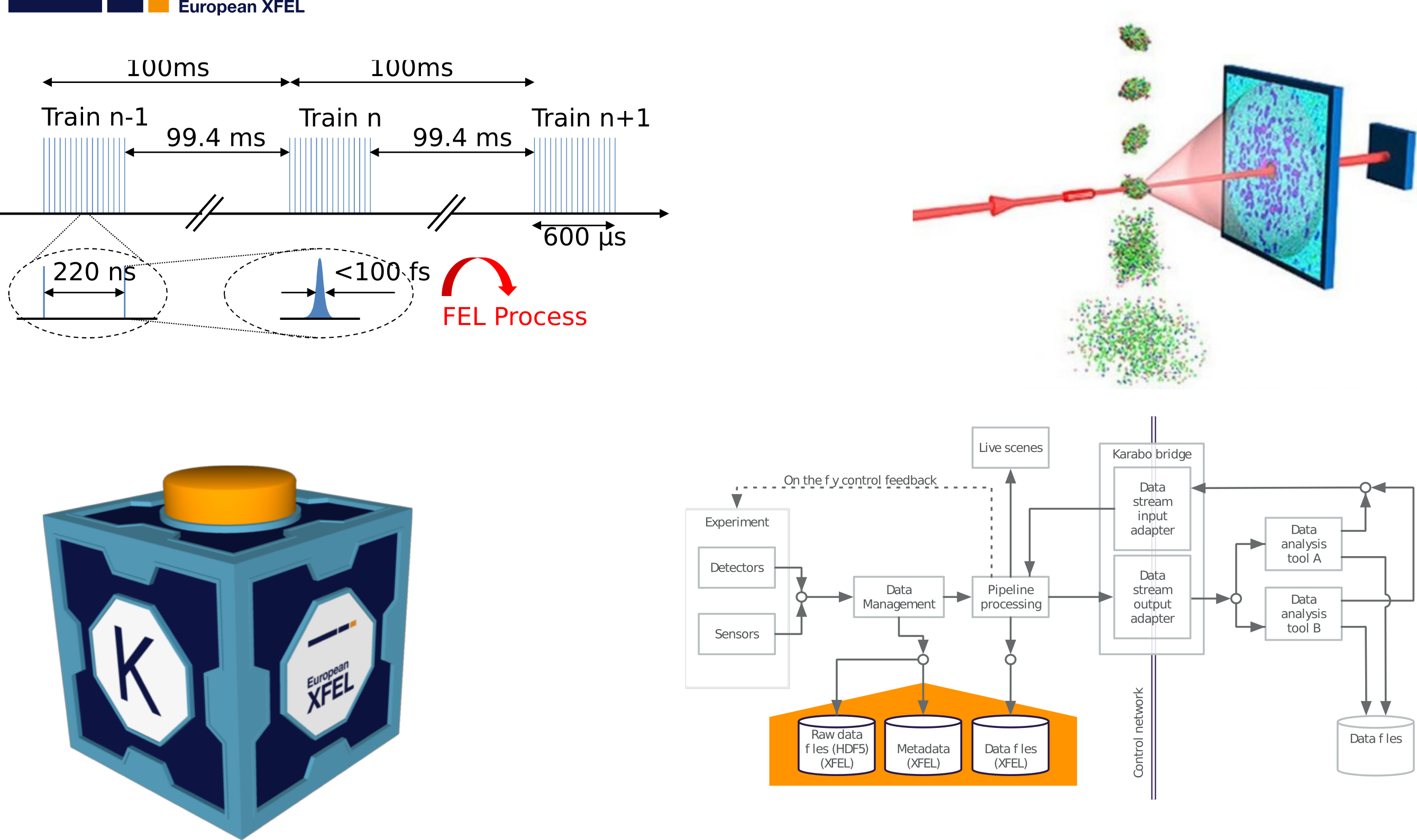
- 09/2018 - present : Software Engineer (Eu XFEL)
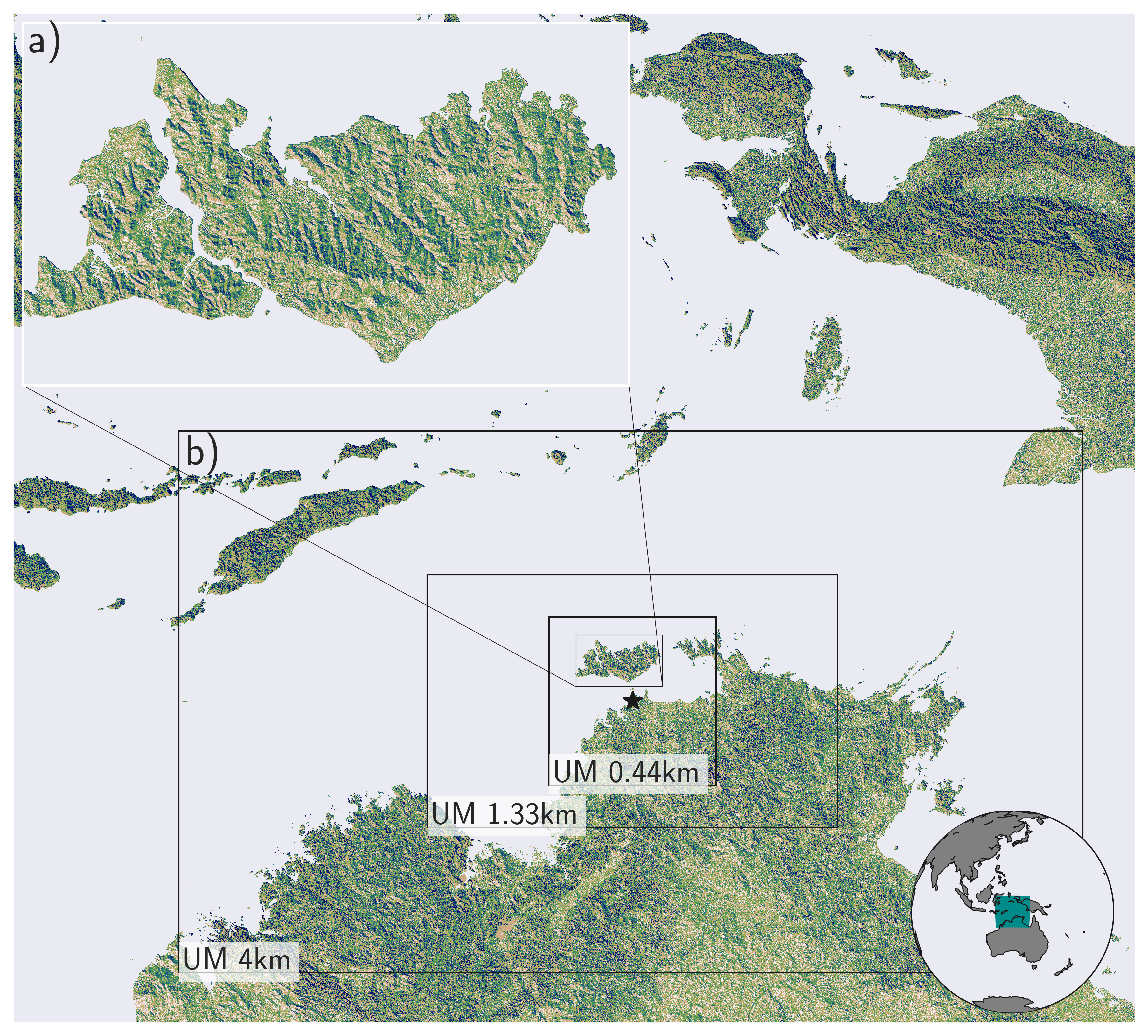
Investigation of Extremes in Island Thunderstorms
In [5]:
%%HTML
<ul>
<li>
<p><font color="#fc1717">4 km</font> → <font color='#1f1a95'>1.33 km</font>→ <font color='orange'> 0.44 km</font>
</li>
<li>80 Vertical Level</li>
<li>8 Ensemble Member, each 6 hours different init time</li>
</p>
</ul>
In [7]:
display(p3plot)
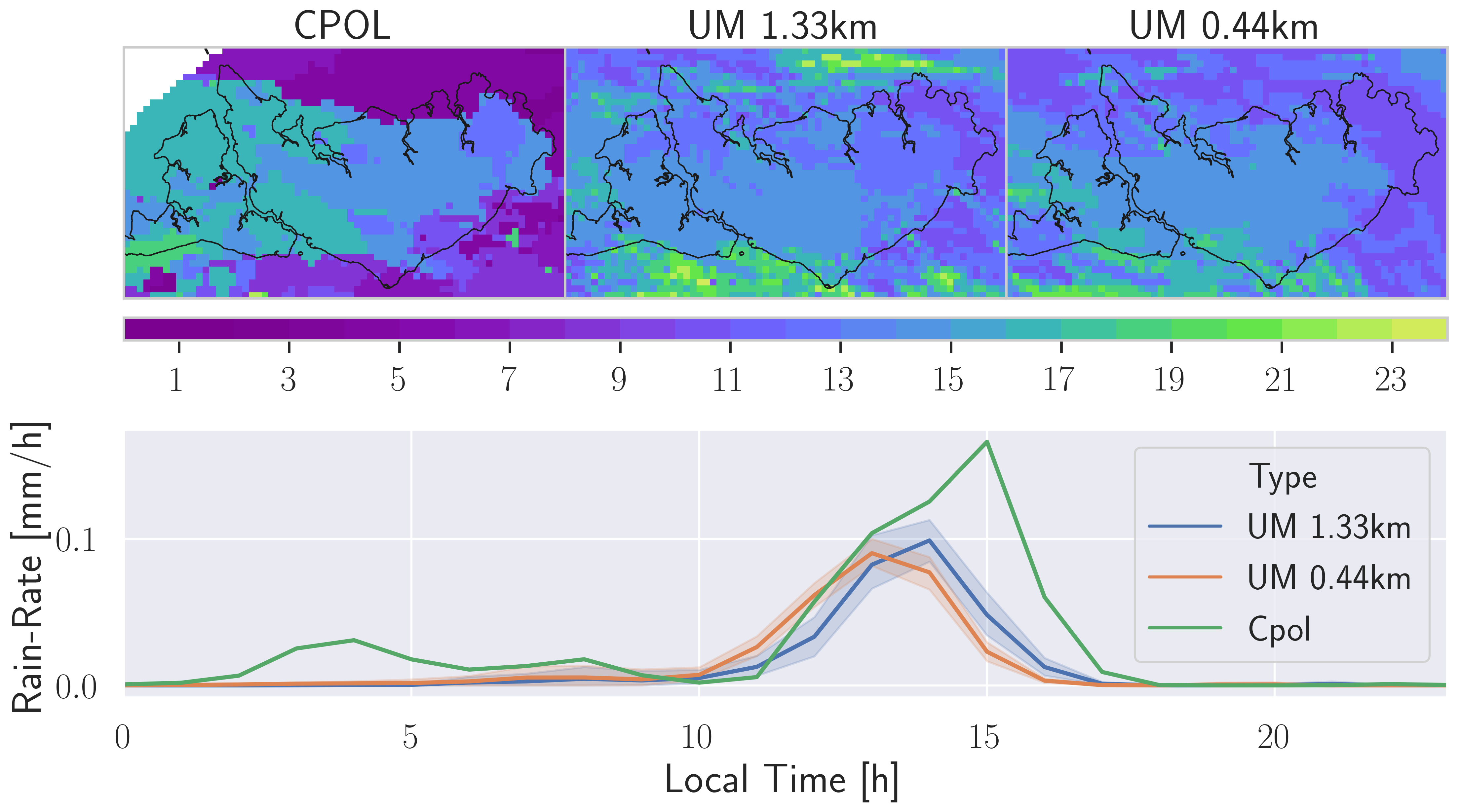
The simulated Diurnal Cycle
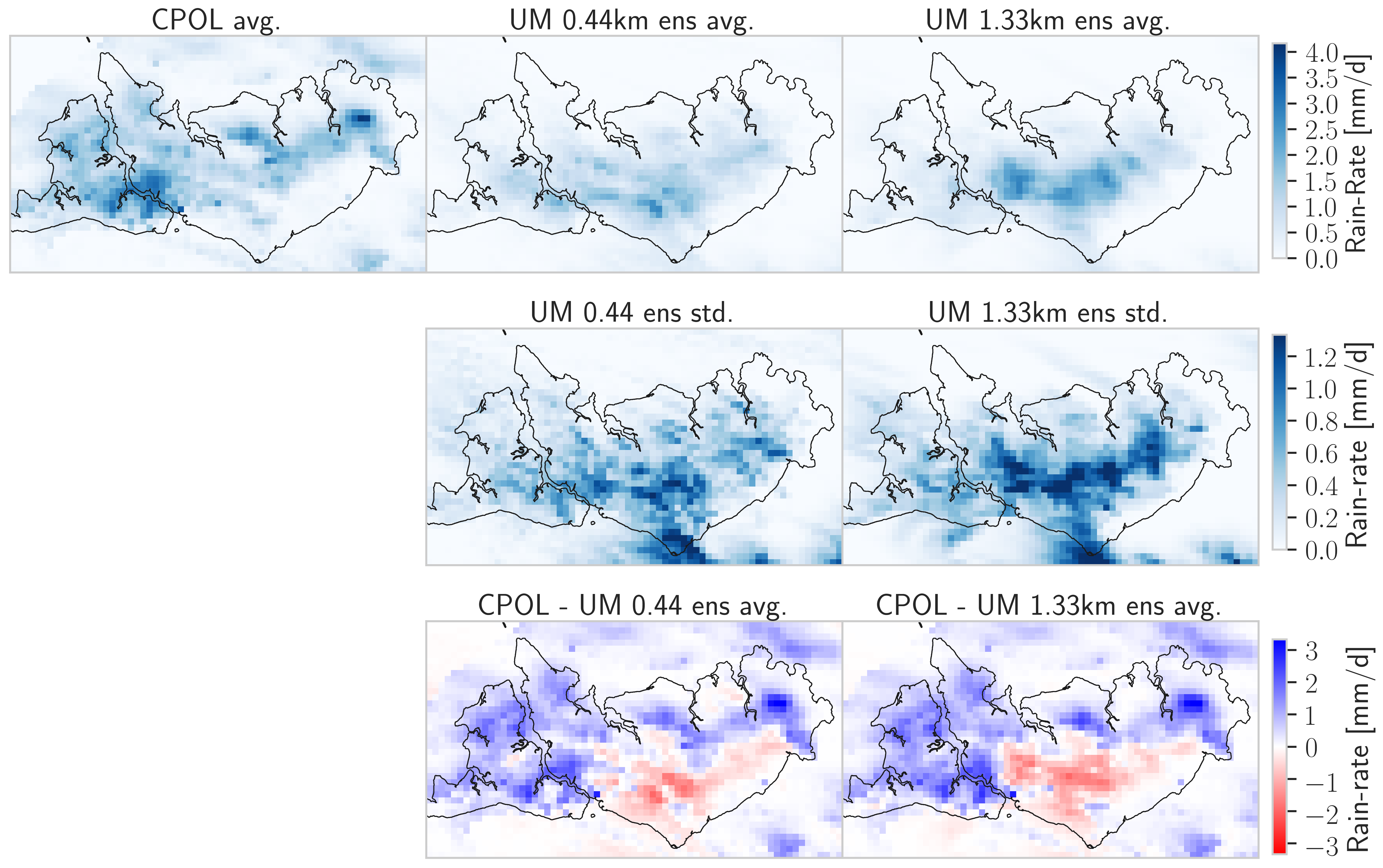
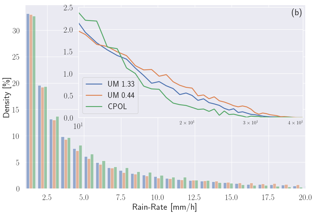
How well are Extremes Represented?
In Summary:
- Storms are a Little too early in the Model
- Occure too Central over Melville Island
- Extreme Events are Slighly Over Estimated
- Slight Improvement with Higher Resolution Version
Storm-Track Analysis
- Analyse Strom tracks using an adopted tracking verion of TINT
- TINT -> Tracking with Phase-Correlation and "Hungarian" similarity mathiching
In [15]:
display(pd.read_pickle('medians.pkl').round(2))
The strongest Stormes (>9th decile)
In [16]:
f =  open('../slides/d3plot_map.dmp','rb')
mapplot = pickle.load(f)
f.close()
display(mapplot)
Storm Properties by Intensity
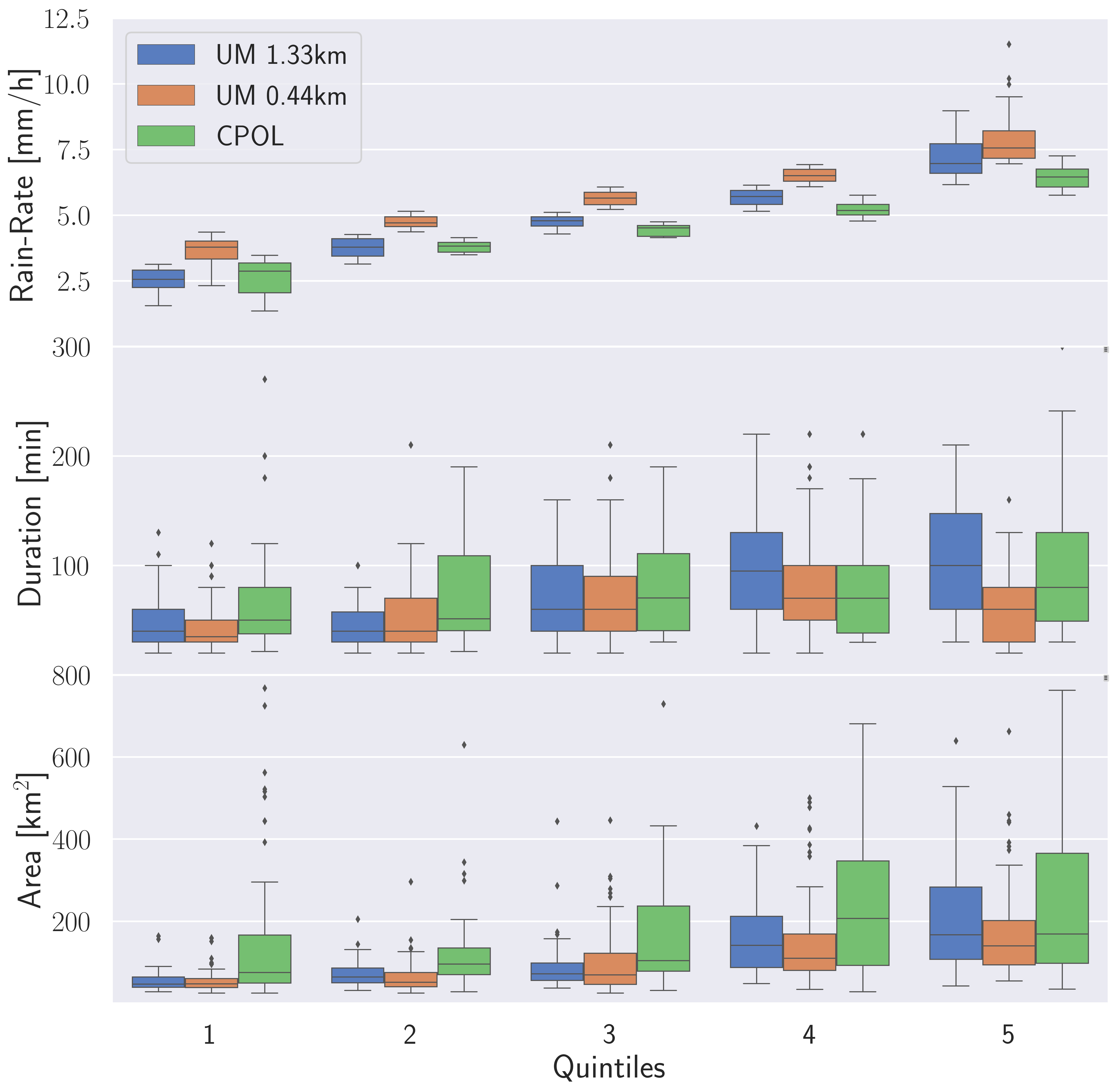
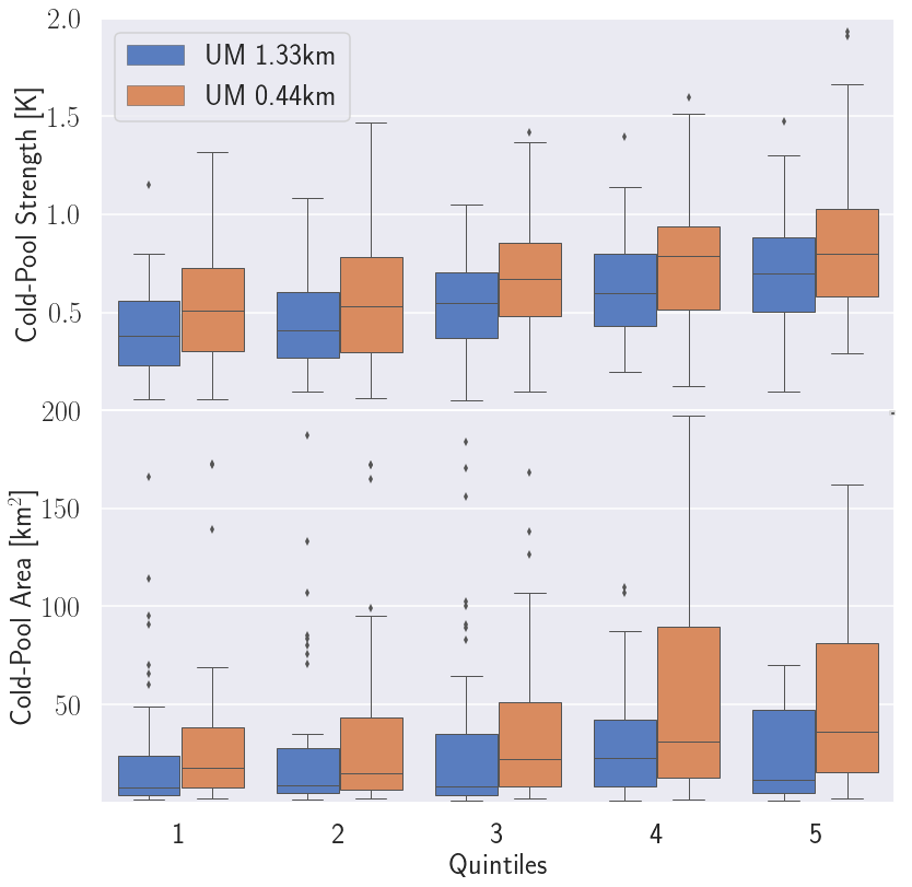
Why are Storms more intense in the Sub-km version?
- Investigation of Cold-Pools
In [19]:
%%HTML
<figure>
<video width="500" loop="true" controls>
  <source src='ColdPool-Ens-1.mp4' type="video/mp4">
</video>
 <figcaption  style="text-align: right">Tracking with Density Potential Temperature Field Pertubation</figcaption>
</figure>
- The State of the Atmosphere
In [22]:
from copy import deepcopy

variables=dict(omega=(("$\\overline{\\omega'}$ [m/s]"), (-9.5e-2, 8.5e-1), 1),
               mflux=("$\\overline{\\omega' q'}$ [m g/kg s]", (-1.2e-1, 1.6), 1000))#
nrow = 0
data = []
fontsize = 18
y_axis_layout=dict( gridcolor='rgb(255,255,255)', showgrid=True, showline=False, showticklabels=True,
                    titlefont=dict(size=fontsize), tickcolor='rgb(127,127,127)', ticks='outside',
                    zeroline=False, range=[P[0], P[-1]])
x_axis_layout=dict( gridcolor='rgb(255,255,255)', showgrid=True, showline=False, showticklabels=True,
                    tickcolor='rgb(127,127,127)', ticks='outside', zeroline=False, titlefont=dict(size=fontsize))
for layout_dict in (x_axis_layout, y_axis_layout):
    layout_dict['tickfont']=dict(size=fontsize-2)
    layout_dict['automargin'] = True

xaxis = {}
yaxis = {}
nplot = 1
nquint = 5
hspace, vspace = 0.01, 0.15
titles = []
colors = ('#1f77b4', '#ff7f0e')
for nvar, (var, prop) in enumerate(variables.items()):
    nrow += 1
    varn, xrange, mul = prop
    for nn, quint in enumerate(range(1,nquint+1)):
        for nrun, (run, flx) in enumerate(fluxes.items()):
            x = flx[var][quint] * mul
            if nrow == 1 :
                yname = 'y'
            else:
                yname = 'y%i'%(nrow*nquint-nquint+1)
            if nplot > 1:
                showlegend=False
            else:
                showlegend=True
            trace = go.Scatter(
                x = x,
                y = P,
                name=run,
                xaxis='x%i'%(nplot),
                yaxis= yname,
                visible = True,
                showlegend = showlegend,
                mode = 'lines',
                line = dict(color = colors[nrun], width = 3)
            )
            data.append(trace)
        yaxis['yaxis%i'%(nplot)] = deepcopy(y_axis_layout)
        xaxis['xaxis%i'%(nplot)] = deepcopy(x_axis_layout)
        xaxis['xaxis%i'%(nplot)]['title'] = varn
        yaxis['yaxis%i'%(nplot)]['domain'] = split(len(variables), vspace)[nrow-1]
        xaxis['xaxis%i'%(nplot)]['domain'] = split(nquint, hspace)[nn]
        xaxis['xaxis%i'%(nplot)]['anchor'] = yname
        yaxis['yaxis%i'%(nplot)]['anchor'] = 'x%i'%nplot
        xaxis['xaxis%i'%(nplot)]['range'] = xrange
        if quint == 1:
            yaxis['yaxis%i'%(nplot)]['title']='Pressure [hPa]'
        if nrow == 1:
            xaxis['xaxis%i'%(nplot)]['range'] = xrange
            sp = split(nquint, hspace)[nn]
            titles.append(dict(x=(xrange[1]-xrange[0])/2 - ((xrange[1]-xrange[0])/20),
                               y=split(nquint, vspace)[-1][-1]+vspace/4,
                               showarrow=False,
                               text='Quintile %i'%quint,
                               xref='x%i'%(nplot),
                               yref='paper'))
        nplot += 1

layout = go.Layout(
    width=750,
    height=800,
    annotations=titles,
    autosize=False,
    paper_bgcolor='rgb(255,255,255)',
    plot_bgcolor='rgb(229,229,229)',
    font=dict(family='serif', size=fontsize, color='#7f7f7f')
)
for axis, axlayout in yaxis.items():
    layout[axis] = axlayout
for axis, axlayout in xaxis.items():
    layout[axis] = axlayout

'''
steps=[]
labels={i: str(i) for i in range(1,6)}
labels[0] = 'All'
for n in range(6):
    step = dict(
        method = 'restyle',
        args = ['visible', [False] * len(data)],
        label=labels[n])
    for ii in range(2):
        step['args'][1][n+ii*6] = True # Toggle i'th trace to "visible"
    steps.append(step)

sliders = [dict(
    active = 5,
    currentvalue = {"prefix": "Quintile: "},
    pad = {"t": 75},
    steps = steps,
    font=dict(size=16)
)]
layout['sliders'] = sliders
'''
fig = go.Figure(data=data, layout=layout)
display(py.iplot(fig, show_link=False))
In [28]:
%%HTML
<figure>
<video width="750" height="350" loop="true" controls>
  <source src='ColdPool_nativ_2.mp4' type="video/mp4">
</video>
 <figcaption  style="text-align: right">Cold-Pool (center) and Rainfall (outer) for two ensemble member</figcaption>
</figure>
<img src="Diagram1.png" alt="Study area" style="height:150px;"/>
<p>One possible problem: Micro-Phys. depends on RH<sub>crit</sub> that is chosen on 80!! levels</p>
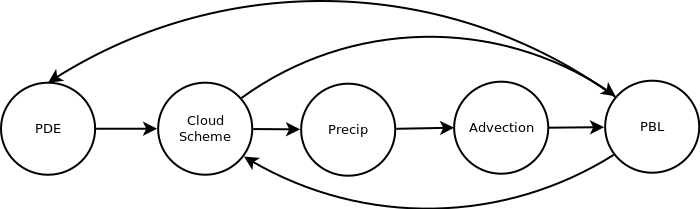
One possible problem: Micro-Phys. depends on RHcrit that is chosen on 80!! levels
In [ ]: